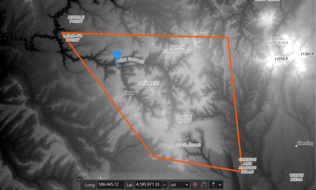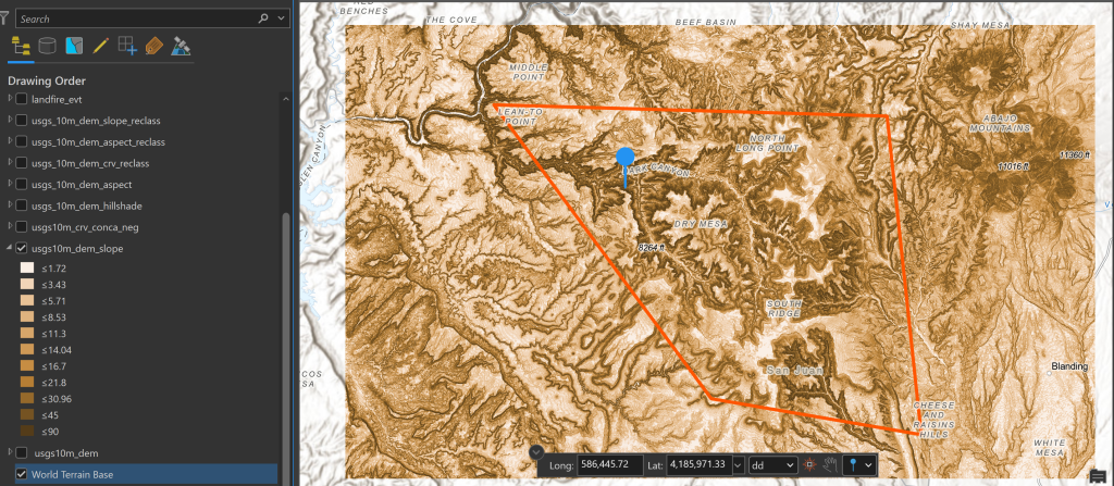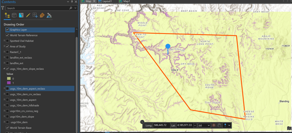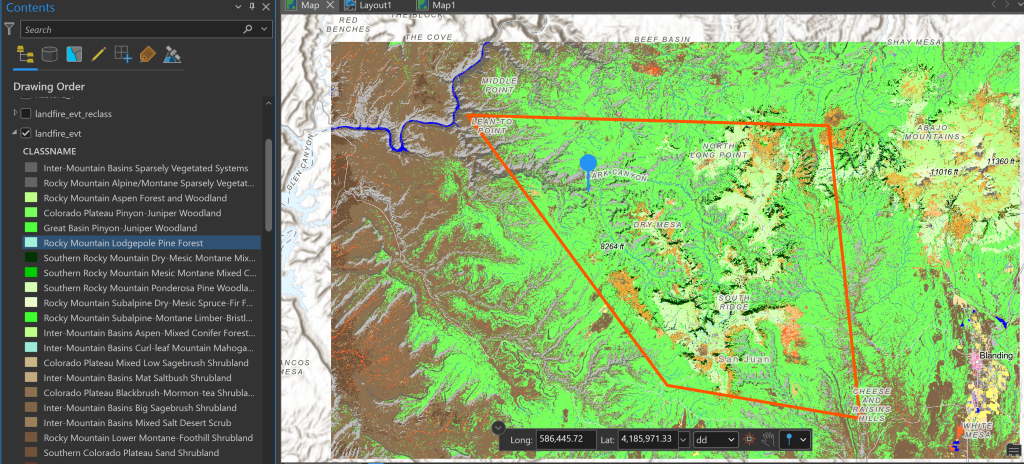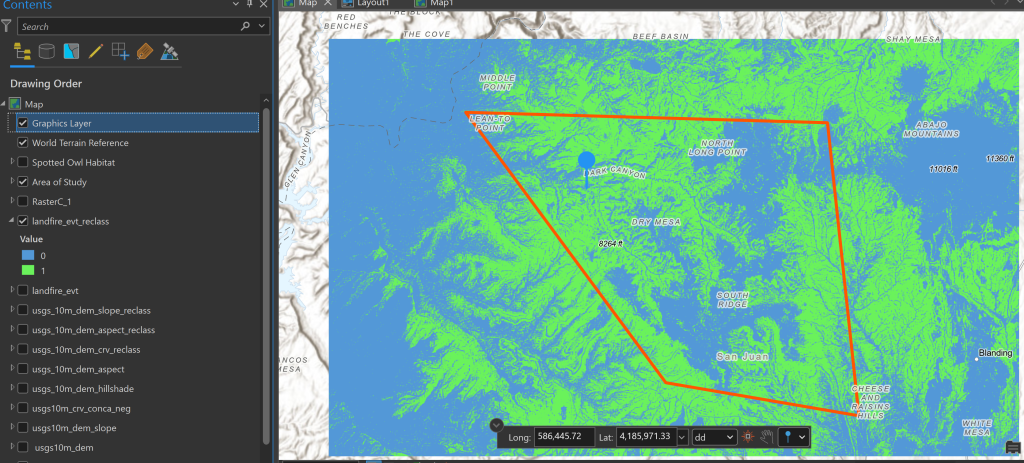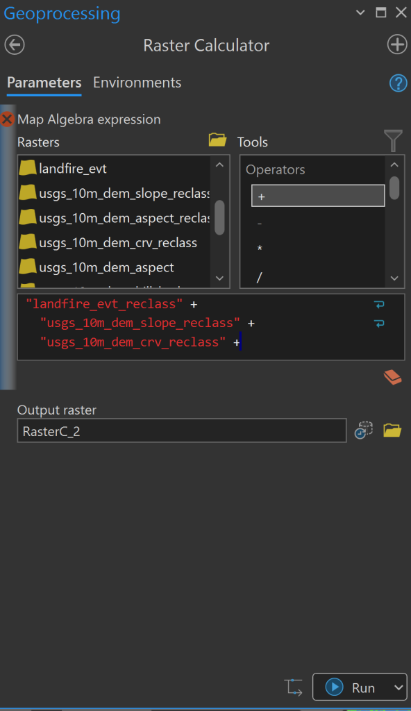
In this post I was learning to combine and manipulate rasters in ArcGIS Pro in order to locate a suitable habitat for the Mexican Spotted Owl in southeastern Utah, in the United States. I found this project interesting not only for the problem at hand, but also the level of complexity. For me, it was one of the most complex projects I’ve tried to date, and gave me a better idea of why naming conventions and data storage processes are important. No use in doing all the work involved if you can’t find the final results file when you’re finished!
General Criteria for Mexican Spotted Owl Habitat
| Layman’s Lingo | GIS Data Variable | Refined Habitat Criteria |
| Vegetation area with trees | Landcover | Pinyon-juniper communities |
| Steep Canyons | Slope | Slopes greater than 40° |
| Ledges & Caves | Concavity/Convexity | Curvature values greater than 1.5 SD from mean |
| Faces mostly North | Aspect | North West, North, and North East aspects |
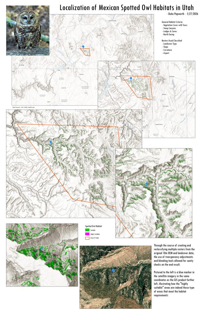
Above is pictured the final product for export or printing at poster-size, but I thought I would add a few more screenshots below showing the process.