
This time we’re taking a look at coyote patterns in part of Utah, working with XY data from radio/GPS collars, and learning more about how to take that data of positions over time to give us an idea of how large or small of a home range these specific animals might have. Along the way we use a bit of python scripting, pull raster values into points, and also work with vegetation types in the area to see what coyotes might have a preference for in terms of vegetation.
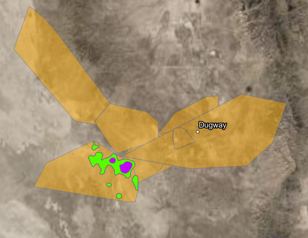
To start off, I’m illustrating below a comparison between two different ways of calculating a home range based on the XY data from the GPS collar positions. In orange we see a less precise, less analytical demonstration of what is called “Minimum Bounding Geometry” in ArcGIS Pro. This takes the XY points from each coyote (there are seven distinct animals present in this data) and draws a polygon to encompass all the pertinent XY points. Interesting to see how far the animals might roam in this way, but not necessarily demonstrative of where they would be most likely or most commonly found on any given day.
The green and purple colored areas superimposed on top of the orange demonstrate a different process, called Kernel Density. Much more statistical, this takes every XY point as the tip of what you might imagine as a three dimensional bell curve, or honestly just imagine a bell. The center of the bell’s vertical axis (right where the bell would hang from) is the location where the coyote is most likely to be, probability-wise, and it becomes less likely to be present in each location on that bell as you move away from center towards the edges.
In the example below, the green colored areas use Kernel Density applied to show where 95% of the coyotes will be present, and the purple areas show where 50% of the coyotes will be present.
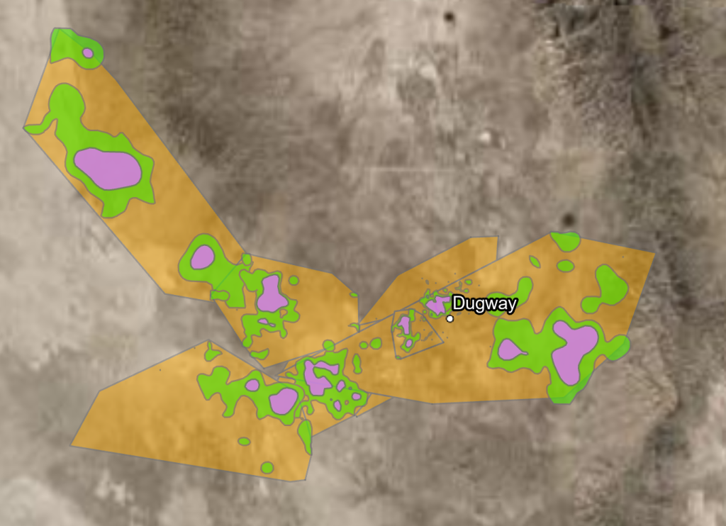
| Type of Home Range | Color on Map | Area of Range (in sq miles) |
| Minimum Bounding Geometry | Orange | 282 |
| General Range (Kernel Density) | Green | 76 |
| Core Range (Kernel Density) | Purple/Violet | 17 |
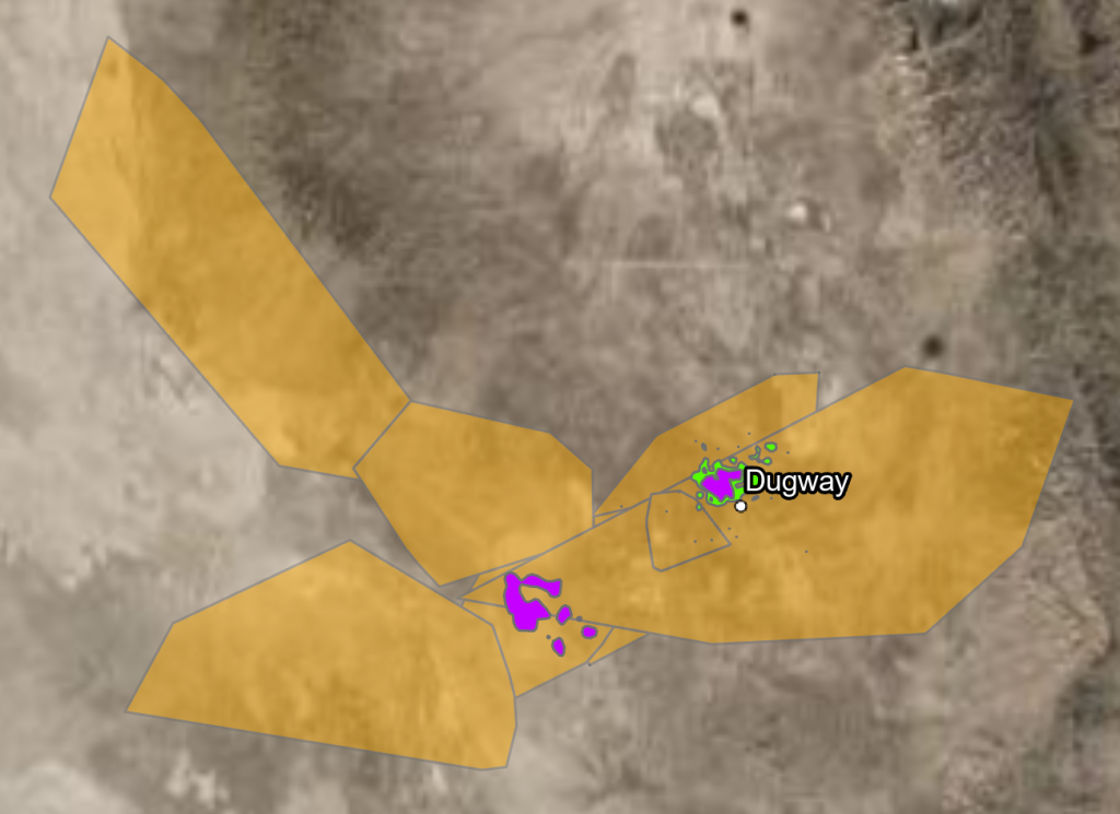
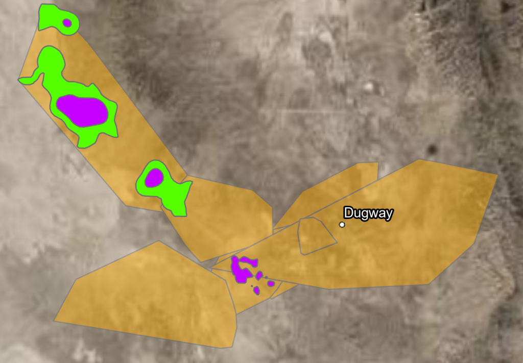
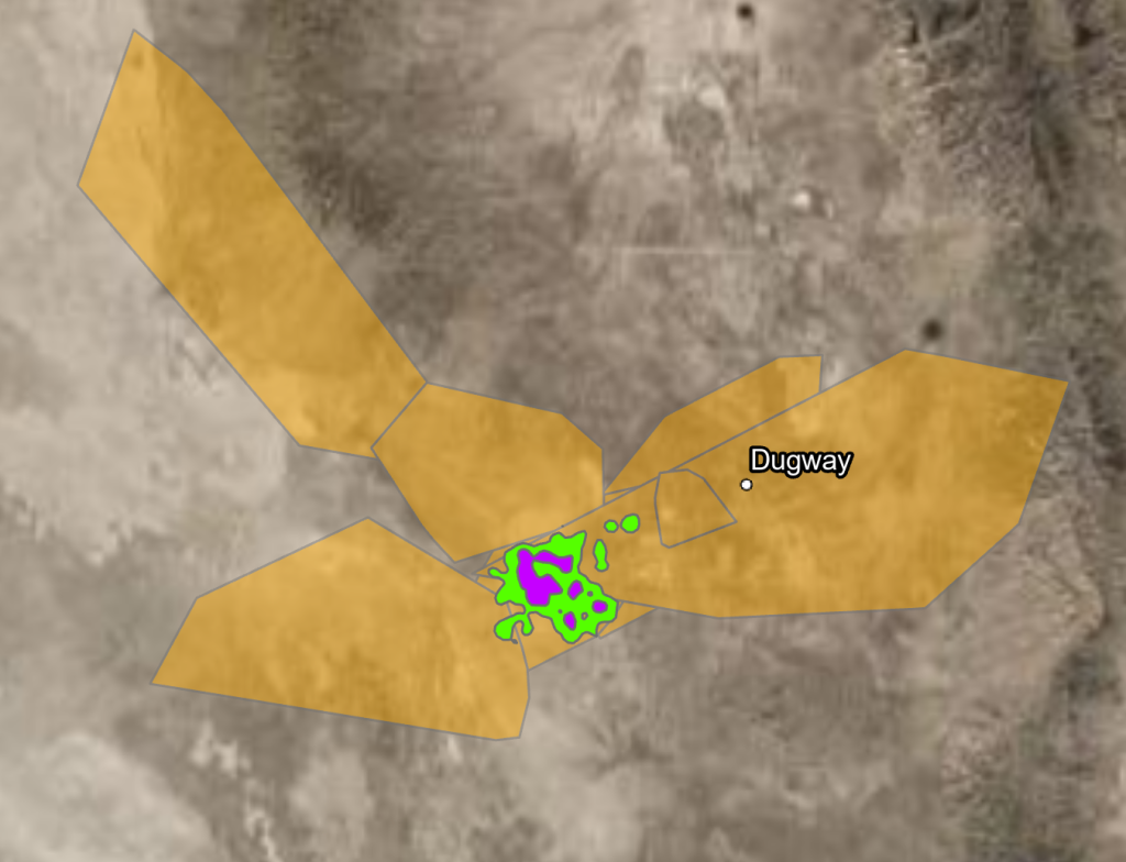
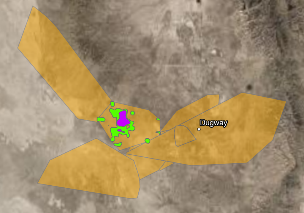
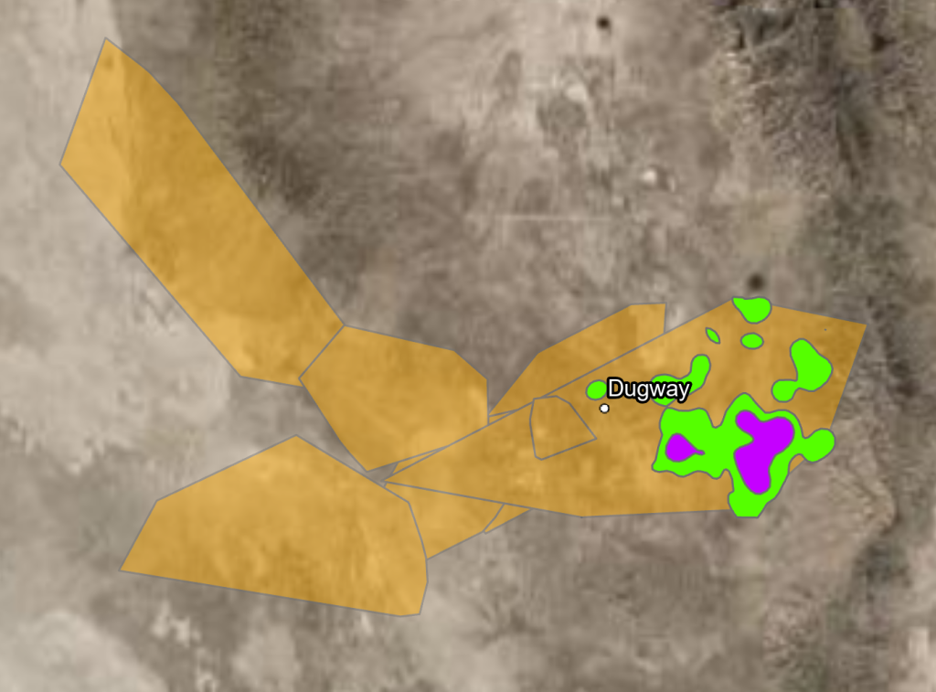
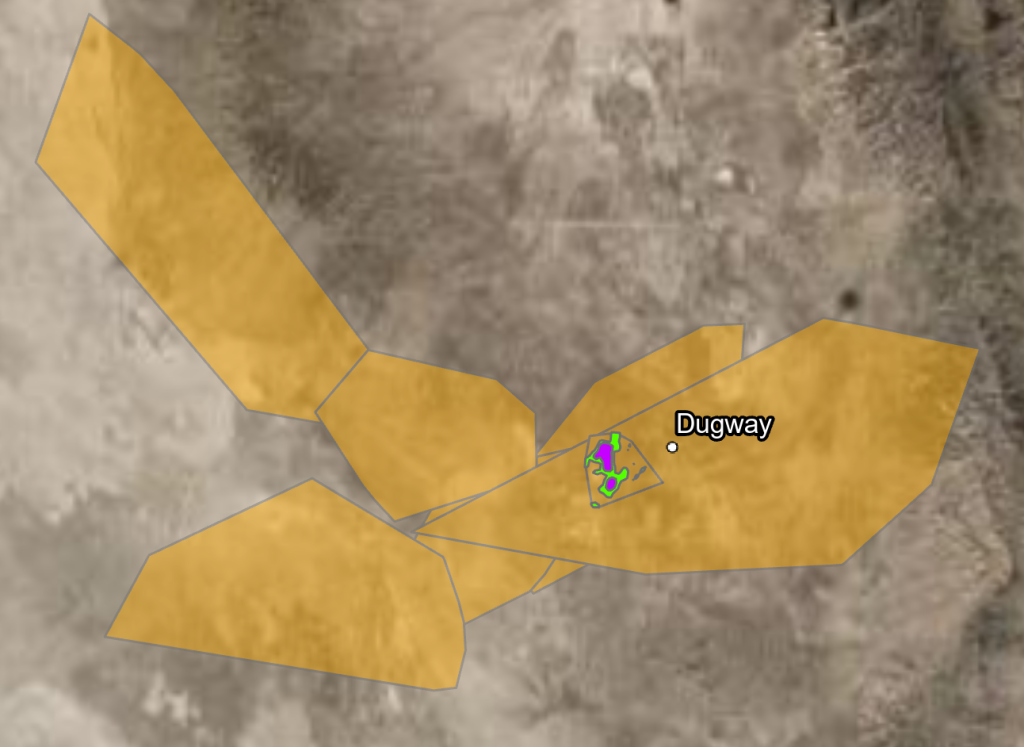
Similar to above, in the images below we can see the Kernel Density process applied to each of these maps in green and purple, with the orange minimum bounding geometry giving a good context of the area. However, in this case, we see the Kernel Density process applied to each individual animal’s XY points in turn, hence the labeling – “animal C02, animal C07, etc.”
Secondary Analysis
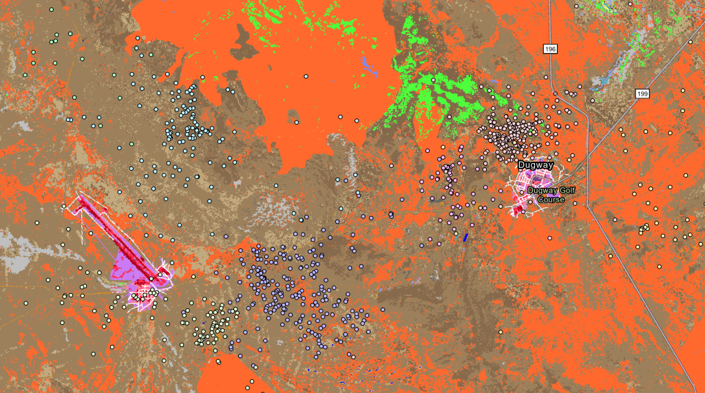
Continuing with much of the same data and adding a bit more, we start to look at the vegetation preferences of the coyotes, as in what types of vegetation do they prefer to exist in, or are they most often found in. Using landcover data for this geographic area and combining it with our previous data, including the XY data points, we can begin to “run the numbers” to get some proportions and try to deduce what type of vegetation coyotes tend to prefer (preference ratio).
After a number of calculations, we end up with a table below:
| How Often Vegetation Type Was “Used” by Coyotes | Vegetation Type | How many units of vegetation type available in study area? | Available Proportion of Vegetation Type | Expected Frequency of Vegetation Use Based on Even Distribution | Preference Ratio – How much was Vegetation preferred compared to anticipated even distribution |
| 7 | Barren | 144895 | .08 | 73 | 0.1 |
| 36 | Great Basin Pinyon-Juniper Woodland | 201907 | .11 | 102 | 0.4 |
| 1 | Inter-Mountain Basins Juniper Savanna | 4133 | 0 | 2 | 0.5 |
| 2 | Western Cool Temperate Developed Ruderal Grassland | 8134 | 0 | 4 | 0.5 |
| 1 | Western Cool Temperate Urban Herbaceous | 3430 | 0 | 2 | 0.6 |
| 1 | Inter-Mountain Basins Semi-Desert Shrub-Steppe | 3136 | 0 | 2 | 0.6 |
| 188 | Introduced Upland Vegetation-Annual Grassland | 551205 | 0.3 | 278 | 0.7 |
| 60 | Great Basin Xeric Mixed Sagebrush Shrubland | 150568 | 0.08 | 76 | 0.8 |
| 1 | Inter-Mountain Basins Sparsely Vegetated Systems II | 2147 | 0 | 1 | 0.9 |
| 3 | Inter-Mountain Basins Big Sagebrush Steppe | 5669 | 0 | 3 | 1.0 |
| 4 | Artemisia tridentata ssp. vaseyana Shrubland Alliance | 7073 | 0 | 4 | 1.1 |
| 70 | Inter-Mountain Basins Big Sagebrush Shrubland | 94653 | 0.05 | 48 | 1.5 |
| 24 | Introduced Upland Vegetation-Annual and Biennial Forbland | 31793 | 0.02 | 16 | 1.5 |
| 420 | Inter-Mountain Basins Mixed Salt Desert Scrub | 513248 | 0.28 | 259 | 1.6 |
| 93 | Inter-Mountain Basins Greasewood Flat | 102117 | 0.06 | 52 | 1.8 |
| 5 | Developed-Roads | 5120 | 0 | 3 | 1.9 |
| 1 | Developed-High Intensity | 817 | 0 | 0 | 2.4 |
| 1 | Inter-Mountain Basins Sparsely Vegetated Systems | 776 | 0 | 0 | 2.6 |
| 2 | Developed-Low Intensity | 1285 | 0 | 1 | 3.1 |
| 5 | Developed-Medium Intensity | 1255 | 0 | 1 | 7.9 |
There is a lot to go over in the data, but from the table above, a few things stand out. Whenever we have a low count of how much a certain vegetation type was used by coyotes, we have to be careful trusting this data. A single point or a few there compared to how much of that vegetation type is available can lead to a very high preference ratio, which really isn’t necessarily true. However, we do see, in the four bolded “Intermountain…” type vegetation types that we have a higher preference ratio, along with plenty of samples from those areas, a larger amount of “uses” by the coyotes. This demonstrates that it is more likely that coyotes do actually prefer this type of vegetation over other types when possible.
Beyond using the GIS specific tools, like ArcGIS Pro, I am understanding more and more about how much analysis and statistical type thinking goes into projects like this. So called “sanity checks” before we plow into the geoprocessing tools can save a lot of time. In this project, realizing that simply having a high preference ratio wasn’t an automatic answer to what coyote’s preferred in actuality was something that made a lot of sense to me but also wasn’t obvious to me at first glance. I’m sure out on the range they’d always recommend “measure twice, cut once” – this is helpful in GIS work too!